These programs were created to provide students with the ability to verify mathematical concepts and answer both visually and numerically. Tutorials for adding the programs to calculators using TI-Connect CE or to the TI-Smartview emulator are at the bottom of the page.
All programs should be run in RADIAN mode.

Program	Description
IROC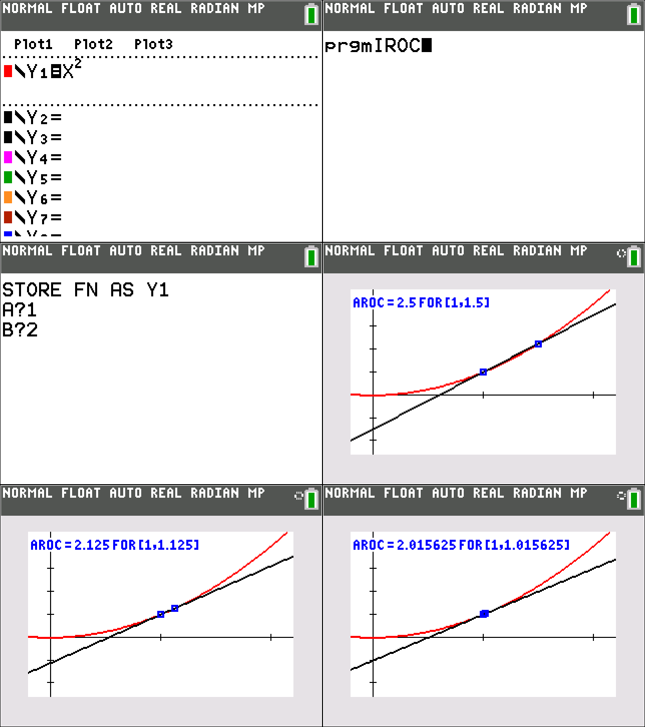 DOWNLOAD	This program demonstrates a secant line in which a point of intersection moves towards the other point of intersection. Enter the function into Y1. Run the program. Enter the x-coordinate for the stationary point of intersection as A. Enter the x-coordinate for the point of intersection which will move towards the first point. The program will automatically size the window, so the first point of intersection is centered. The graph of the function will be displayed between with a secant intersecting the graph at x=A and x=B. The slope of the secant line will be displayed at the top of the screen. The program will then be paused until ENTER is pressed. (A small “gear” will be displayed next to the battery in the upper right corner when the program is paused.) After ENTER is pressed, the program will redraw the secant line so that width of the previous interval is divided by 10. The program will display a total of 4 different secant lines. The window for the graph never changes.
IROC ZOOM DOWNLOAD	This program demonstrates a secant line in which the a point of intersection moves towards the other point of intersection. Enter the function into Y1. Run the program. Enter the x-coordinate for the stationary point of intersection as A. Enter the x-coordinate for the point of intersection which will move towards the first point. The program will automatically size the window, so the first point of intersection is centered. The graph of the function will be displayed between with a secant intersecting the graph at x=A and x=B. The slope of the secant line will be displayed at the top of the screen. The program will then be paused until ENTER is pressed. (A small “gear” will be displayed next to the battery in the upper right corner when the program is paused.) After ENTER is pressed, the program will redraw the secant line so that width of the previous interval is divided by 10. The program changes the window so that the two points of the secant line remain stationary in the display. (The program is zooming the window into the interval displayed to show the local linearity of the curve.) The program will display a total of 4 different secant lines.
TANGENT LINE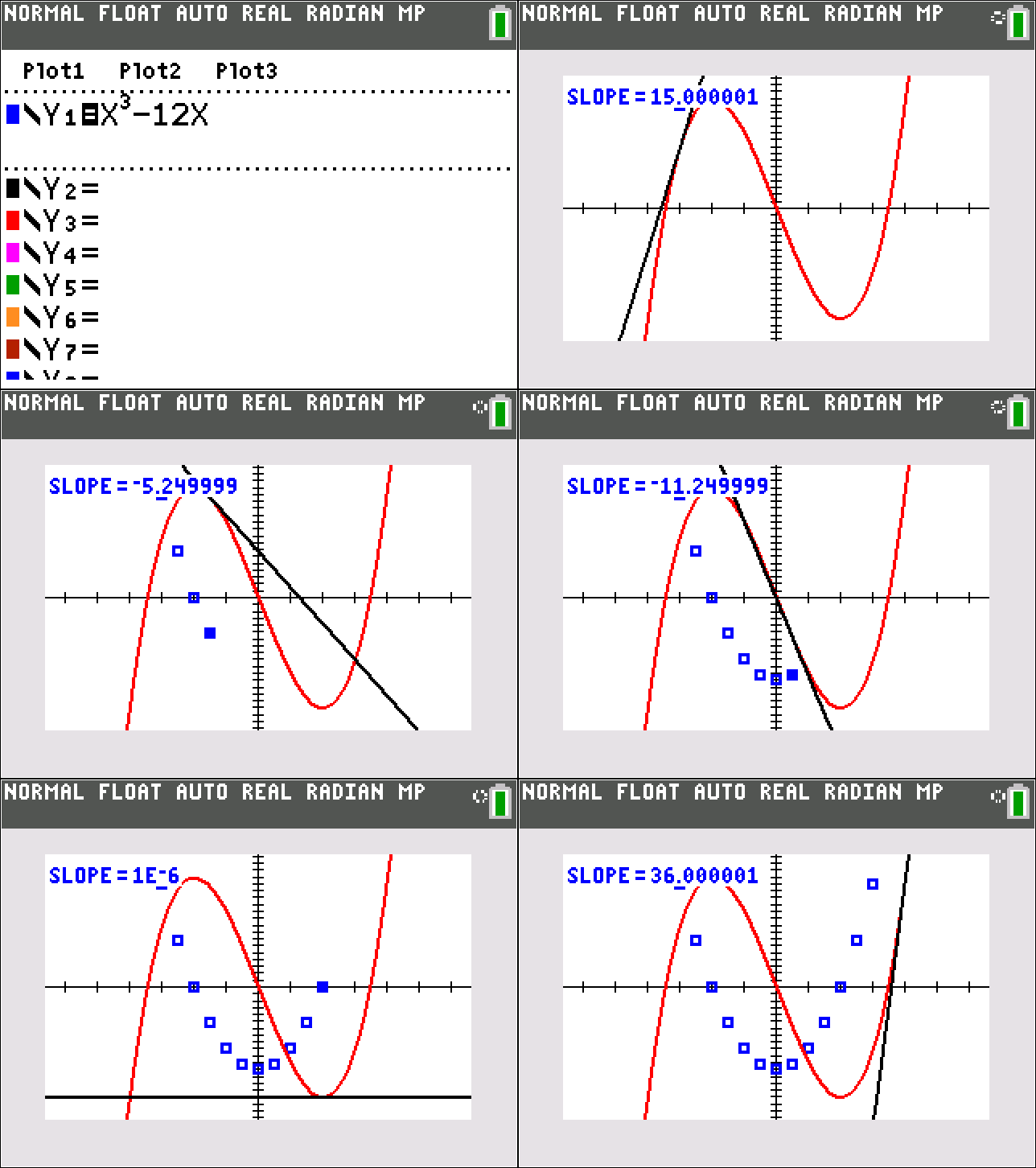 DOWNLOAD	The program then computes the slope for the line tangent to the curve at a particular value of x and uses it to graph a tangent line at the same value. It also plots a point whose x-coordinate is this value of x and whose y-coordinate is the slope of the tangent line. The program then pauses until the user presses enter. The program then moves on to the next x value. The program divides the x interval of the window into 16 pieces, sketching the tangent line and plotting the derivative at each value of x. At the end, the user will have a graph of the function and selected values of the derivative of the function displayed on the screen. I recommend that teachers choose a window to appropriately display their function and store it as a GDB to send to students.
MVT Guess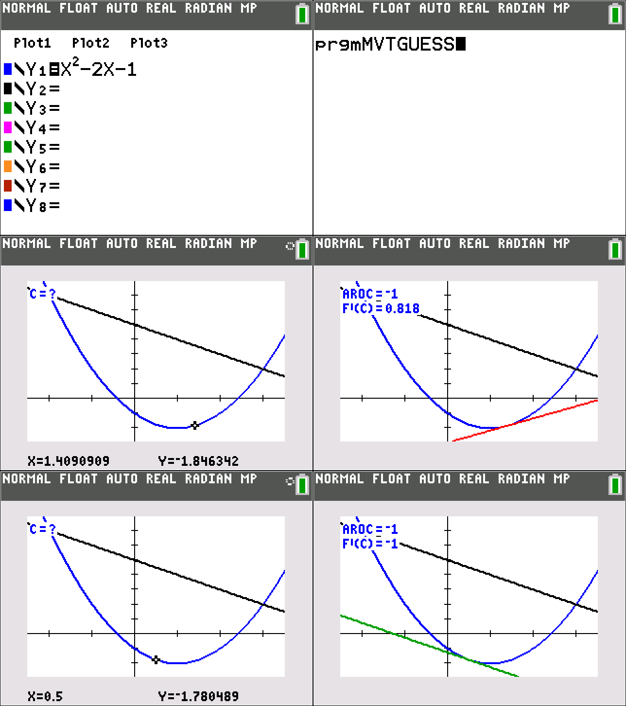 DOWNLOAD	This program lets students graphically guess the x-coordinate of which satisfies the conclusion of the Mean Value Theorem. First enter the function into Y1. Run the program and enter the values of A and B as prompted. The program will automatically sets the window and the graph the function and the secant line from x=A to x=B. The program then allows the user to use the arrow keys to move the flashing cursor to the point where a line tangent to the function will be parallel to the secant line. The program will then draw a line tangent at the x-coordinate of the guess. If the tangent line is parallel, (that is, the x-coordinate satisfies the conclusion of the Mean Value Theorem) then it will be drawn in green. If not, the tangent line will be drawn in red.
MVT Check DOWNLOAD	This program lets students numerically check the x-coordinate which satisfies the conclusion of the Mean Value Theorem. First enter the function into Y1. Run the program and enter the values of A and B as prompted. The program will then prompt the user for the value C which satisfies the Mean Value Theorem for the given interval. The program will automatically set the window and then graph the function, the secant line from x=A to x=B, and the line tangent to the function at x=C. If the tangent line is parallel, (that is, the x-coordinate satisfies the conclusion of the Mean Value Theorem) then it will be drawn in green. If not, the tangent line will be drawn in red.
Riemann Sums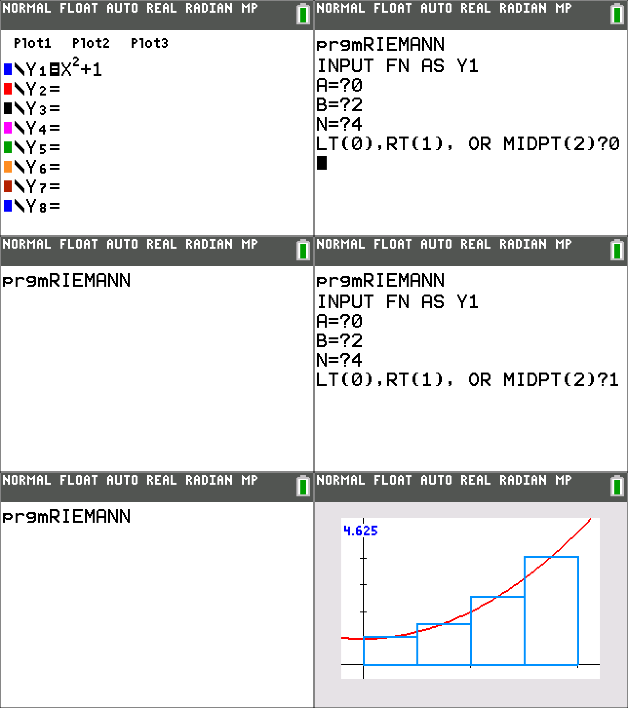 DOWNLOAD	Input the functions into Y1. Run Program and input the lower bound as A and upper bound as B when prompted. Input the number of rectangles of equal width desired. Choose the number corresponding with the type of Riemann Rectangular Approximation Method of your choice. The program automatically resizes the window, displays the graph with the given number of rectangles, and shows the value of the approximation for the integral using the prescribed method.
Trapezoidal Sums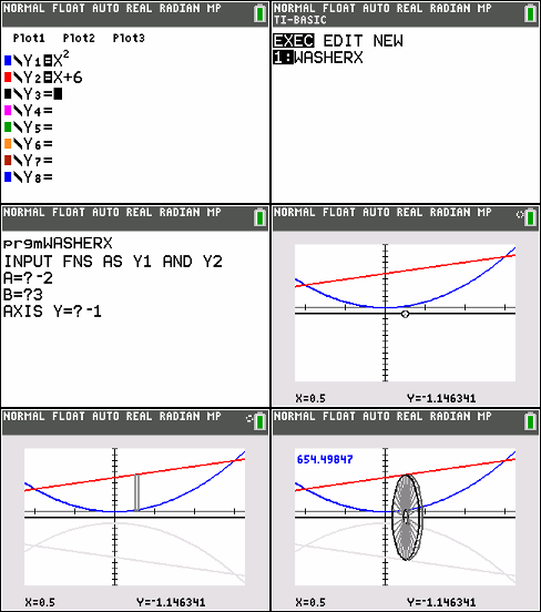 DOWNLOAD	Input the functions into Y1. Run Program and input the lower bound as A and upper bound as B when prompted. Input the number of trapezoids of equal width desired. The program automatically resizes the window, displays the graph with the given number of trapezoids, and shows the value of the approximation for the integral using the trapezoidal sum.
MVT for Integrals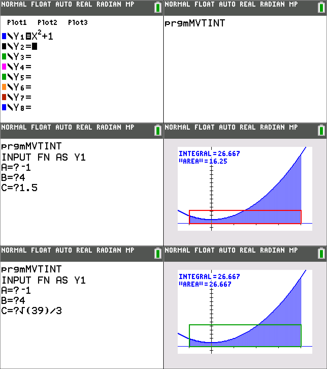 DOWNLOAD	This program lets students numerically check the x-coordinate which satisfies the conclusion of the Mean Value Theorem for integrals. First enter the function into Y1. Run the program and enter the values of A and B as prompted. The program will then prompt the user for the value C which satisfies the Mean Value Theorem for Integrals for the given interval. The program will automatically set the window and then graph the function. It will shade the definite integral over the interval and draw a rectangle whose width is the interval and whose height is the value of the function evaluated at x=C. If the “area” of the rectangle equals the value of the definite integral, (that is, the x-coordinate satisfies the conclusion of the Mean Value Theorem for Integrals) then it will be drawn in green. If not, the rectangle will be drawn in red.
Bounded Area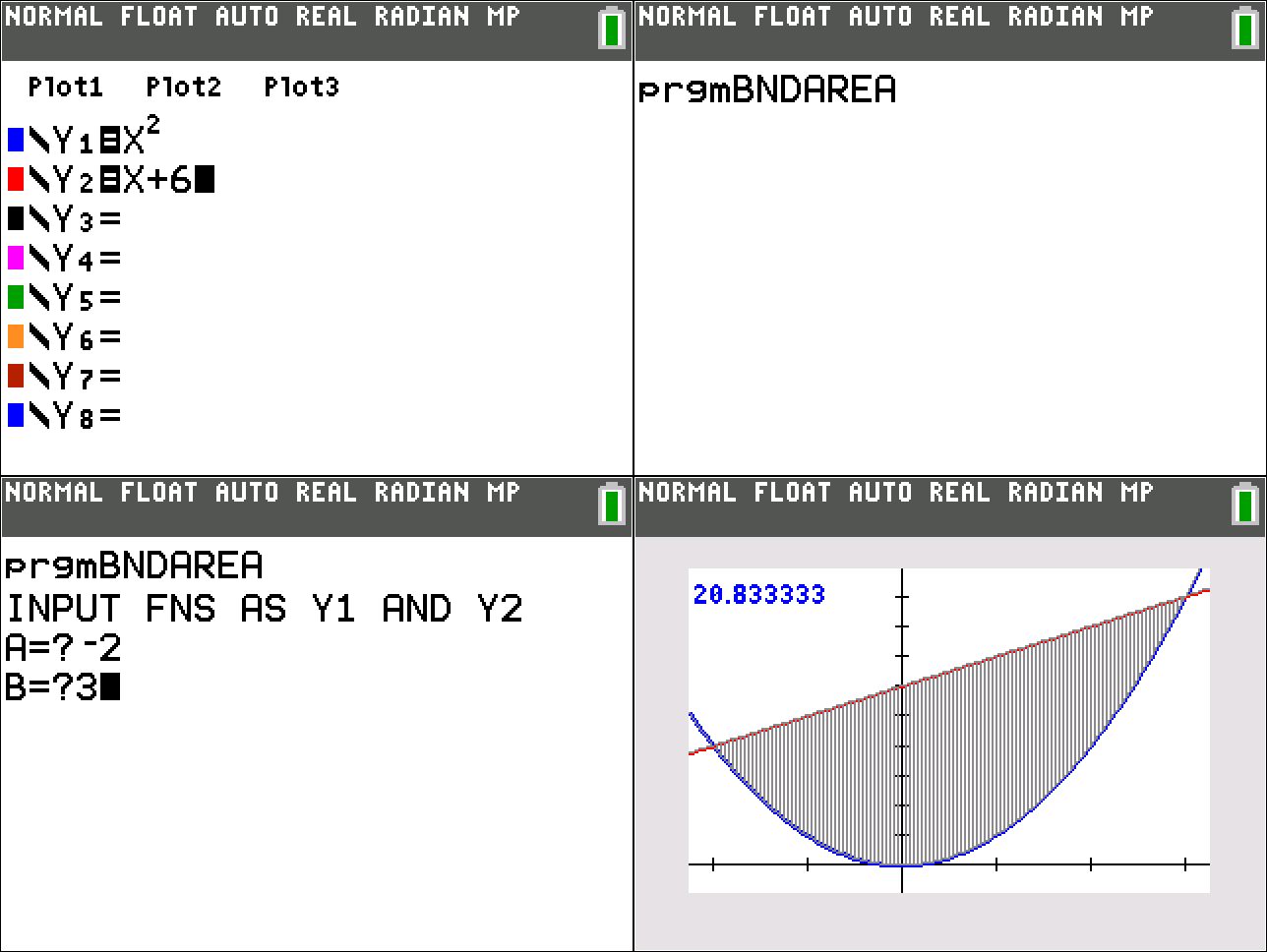 DOWNLOAD	Input functions into Y1 and Y2. Run Program and input the lower bound as A and upper bound as B when prompted. The program automatically resizes the windows, shades the appropriate area, and then displays the numerical approximation of the area. The approximation uses fnint(.
Slope Fields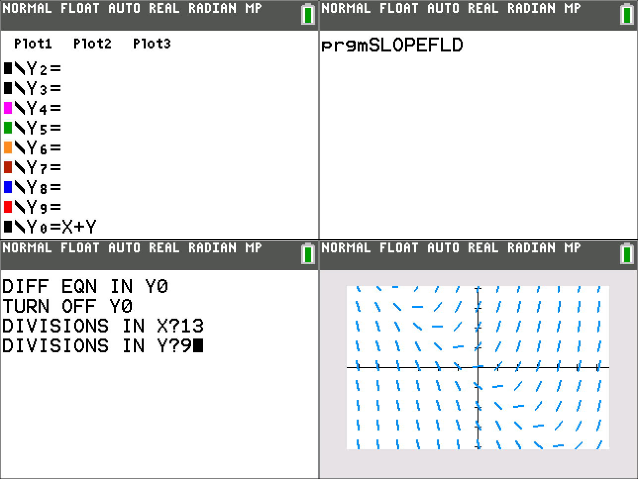 DOWNLOAD	The differential equation should be entered into Y0 as if Y0 were y’. The equation for Y0 must then be turned off. Set the window to your needs. Run the program. Enter the number of line segments you want in each direction. The program will graph the slope field. Particular solutions can be entered for any other equation Y1-Y9 before running the program.
Euler’s Method DOWNLOAD	The differential equation should be entered into Y0 as if Y0 were y’. The equation for Y0 must then be turned off. Run the program. Enter in the coordinate for the initial value when prompted. Enter the step size and the numbers of steps. Enter 0 or 1 to choose if a slopefield should be plotted. The program generates all intermediate values from Euler’s Method and stores them in L1 and L2. The program then turns on Plot1 showing the connected scatterplot of these values in a window set to ZoomData, with or without a slope field. The values can then be viewed by pressing TRACE. When work is concluded, turn off Plot1 manually.
Washer Method X DOWNLOAD	This program draws one washer for the revolution of a region around a horizontal axis. The user should enter the two functions that bound the region from above and below into Y1 and Y2. Once the program is run, it will prompt the uses for the two x values, A and B, which bound the region. It will also prompt for the horizontal axis of rotation. The program then computes the window size which fits the entire region and its reflection over the horizontal axis into the window. It graphs the region and the horizontal axis and pauses. At this point the user should move the cursor left or right to the horizontal position where the washer should be drawn and then press enter. The program then draws a reflection of the region over the axis of rotation in gray and a rectangle whose rotation will generate the washer. The user should press enter once again and the program will draw the washer by rotating the rectangle around the axis of rotation.
Washer Method Y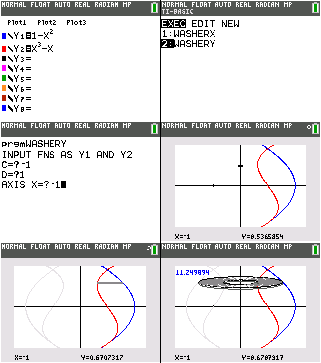 DOWNLOAD	This program draws one washer for the revolution of a region around a vertical axis. The two functions that bound the region to the left and right might by x=f(y) and x=g(y). The user should enter these two functions into Y1 and Y2 such as Y1=f(x) and Y2=g(x). The program will use these functions to graph x as a function of y. Once the program is run, it will prompt the uses for the two y values, C and D, which bound the region. It will also prompt for the vertical axis of rotation. The program then computes the window size which fits the entire region and its reflection over the vertical axis into the window. It graphs the region and the vertical axis and pauses. At this point the user should move the cursor up or down to the vertical position where the washer should be drawn and then press enter. The program then draws a reflection of the region over the axis of rotation in gray and a rectangle whose rotation will generate the washer. The user should press enter once again and the program will draw the washer by rotating the rectangle around the axis of rotation.

Video Tutorial for TI-Smartview CE

Video Tutorial for adding programs to the TI-84 CE Plus using TI-Connect CE

Download TI-Connect CE by clicking here